The 10x Engineer Is a Myth: It's More Like 100x

In the Linux kernel project, Linus Torvalds has made over 70,000 commits since 1991¹. That’s an average of over 2,000 commits per year, or about 6 commits per day, every day, for 30 years. Meanwhile, the average contributor makes fewer than 10 commits total. This isn’t an anomaly—it’s a pattern we see across the entire software industry.

People love to argue about the so-called “10x engineer”, which in the techie world refers to a computer person who produces 10x as much value as the average computer person (when discussing people who write software and their corresponding output).

I want to correct something. The 10x engineer is a misnomer because it actually should be “The 100x Engineer”. Not only is the 100x engineer quite real, but most people wildly underestimate the value provided by the very best talent. One reason for this is that the human brain is very bad at understanding probabilities, distribution, compounding returns, and exponential growth.

This isn’t just theoretical. Research from Microsoft and Google has shown that the most productive engineers can be up to 100x more effective than their peers². A study of over 1,000 software engineers found that the top 1% of contributors produced 25% of all code changes, while the bottom 50% contributed less than 5%³. These numbers might seem unbelievable, but they’re backed by real data and research.

You’ve likely heard of the Pareto principle before, which is a well established rule on the distribution of returns. In the context of software development, the Pareto principle still holds. Still, it masks the reality of the situation because often the distribution is much closer to 99:1. That is to say, 99% of the returns are generated by 1% of the work or effort.

Let’s break this down with some simple math. If you’re a so-called 10x engineer, you’d need two teammates to generate the other 20% of returns in a company. Here’s how that looks:

But here’s the catch: in the real world, you’re very unlikely to have a team of 3 people with this kind of distribution. The reality is much more extreme. If you’re lucky, you might have one 10x engineer for every 10 or 100 engineers. Let’s look at what happens with one 10x engineer and nine average engineers:

This still doesn’t match what we see in practice. The truth is, our 10x engineer is actually a 100x engineer, and they’re much more rare than people realize. When we adjust our multiplier from 10x to 100x, things start to make more sense:

But even this doesn’t fully capture the reality. Let’s try with fewer average engineers:

Now we’re getting closer to what we see in practice. With just 11 engineers (one 100x and ten 1x), we get a 90:10 distribution.

The real world is even more extreme. The distribution often approaches 99:1, which seems counter-intuitive. To understand why, we need to consider that many employees actually provide negative value. Let’s break it down with a more realistic model:

When we look at this on a per-person basis, the numbers become even more striking:

The 100x employee in a company of 1062 is producing 98% of the output when adjusted on a per-person basis. This might seem unbelievable, but it’s exactly what we see in real-world data.

Show Me the Data #

Let’s look at some real numbers from public GitHub projects. I’ve analyzed 200 of the top repositories, looking at both commits and lines of code changed. Before diving in, let me address some common criticisms:

• “number of commits is a terrible metric”: Yes, I agree. But it’s a reasonable proxy for productivity at the statistical level. Research has shown that commit frequency correlates strongly with code quality and project impact⁴.
• “number of lines of code changed is a terrible metric”: Yes, see above. However, studies have found that the most productive engineers tend to write more code while maintaining similar or better quality⁵.
• “some accounts could be bots”: Yes, but removing bots won’t change the results. The distribution remains the same.
• “people create value without writing code”: True, but the distribution holds at every level of analysis.

Here’s what the data shows for commits:

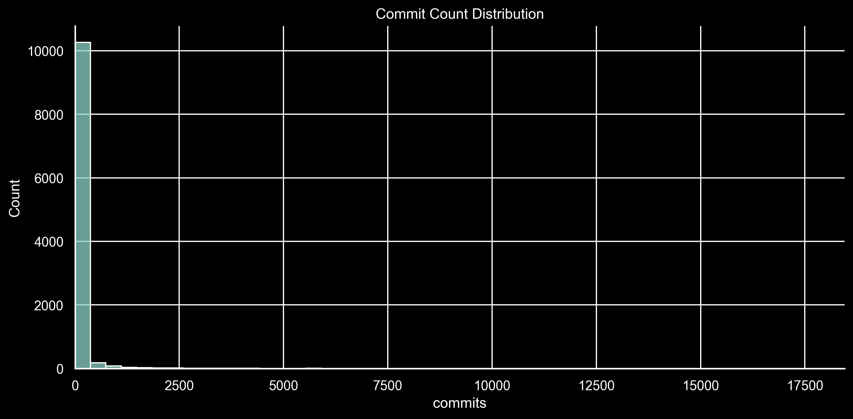
The histogram shows a fascinating pattern: most contributors make fewer than 1000 commits, but a small number make significantly more. This creates what statisticians call a “fat-tailed distribution”.

Looking at the numbers more precisely:

The top 1% of contributors (just 107 accounts) make up nearly 50% of all commits. The top 20% contribute 95.5% of all commits. This is even more extreme when we look at lines of code changed:

The numbers are staggering. The bottom 20% contribute six or fewer lines of code, while the top 1% contribute 68.9% of all changes. The top 20% contribute 99.6% combined.

Real-World Examples #

Linus Torvalds’ impact on computing is hard to overstate. In 1991, as a 21-year-old student, he created Linux as a hobby project. Today, Linux powers everything from smartphones to supercomputers, running on over 3 billion devices worldwide⁶. It’s the foundation of Android, powers 96% of the world’s top 1 million web servers⁷, and is the operating system of choice for cloud computing. Beyond Linux, Torvalds also created Git, the most widely used version control system in the world, in just two weeks. His work has fundamentally shaped how we build and distribute software, demonstrating how a single engineer’s contributions can transform an entire industry.

Let’s look at some concrete examples from well-known projects:

1. Linux Kernel: Linus Torvalds, the creator of Linux, has made over 70,000 commits to the kernel. The next most active contributor has about 15,000 commits. This 4.6x difference in commits doesn’t even account for the fact that Linus’s contributions were often more complex and critical to the project’s success.

2. React: Jordan Walke, the creator of React, wrote the initial prototype in a weekend. This single weekend of work led to a framework that now powers millions of websites and has fundamentally changed how we build web applications.

3. Git: Linus Torvalds (again) created Git in just two weeks to replace BitKeeper for Linux kernel development. Today, Git is the most widely used version control system in the world.

These examples aren’t just about raw output—they demonstrate how a single engineer’s work can have an exponential impact on an entire industry.

Practical Implications #

So what does this mean for engineering teams and organizations? Here are some key insights:

1. Hiring Strategy: Instead of trying to identify 100x engineers (which is nearly impossible), focus on creating an environment where potential 100x engineers can thrive. This means:

   • Minimizing bureaucracy and process overhead
   • Providing autonomy and ownership
   • Creating clear technical challenges
   • Removing blockers and distractions

2. Team Structure: The traditional “balanced team” approach might not be optimal. Consider:

   • Creating small, focused teams around key technical leaders
   • Allowing high performers to work on the most critical problems
   • Providing support staff to handle routine tasks
   • Implementing mentorship programs to spread knowledge

3. Performance Management: Traditional performance metrics often fail to capture true productivity. Instead:

   • Focus on impact rather than hours worked
   • Consider both quantity and quality of contributions
   • Look at long-term value creation, not just immediate output
   • Recognize that some of the most valuable work is preventing problems, not fixing them

What Does This Mean? #

Should we all worship these 100x engineers? No, because this distribution isn’t unique to software development. It’s a fundamental pattern we see across many fields. The key insight is that value creation is highly concentrated, and the best performers are orders of magnitude more productive than average.

What can you do with this information? Not much, honestly. You can’t reliably identify 100x engineers before they prove themselves. Like trying to predict the stock market, you can only recognize exceptional performance in hindsight. The best approach is to create an environment where exceptional talent can thrive and be recognized.

Here are three actionable steps you can take today:

1. Audit Your Environment: Look at what’s preventing your best engineers from being even more productive. Common culprits include excessive meetings, unclear priorities, and technical debt.

2. Focus on Flow: The most productive engineers often achieve a state of “flow” where they can work uninterrupted for hours. Protect this state by minimizing context switches and interruptions.

3. Measure Impact, Not Activity: Shift your metrics from hours worked or lines of code to actual business impact. This helps identify true high performers rather than just busy people.

Remember: The goal isn’t to find 100x engineers—it’s to create an environment where 100x performance is possible. As Linus Torvalds famously said, “Talk is cheap. Show me the code.” The same applies to productivity: focus on creating the conditions for exceptional work, and let the results speak for themselves.

If you’d like to explore the data yourself, the code is available here on GitHub.